KVStore

IKVS Series

在看过《C++ 新经典》后，被其繁杂的特性及语法小小的震撼到了，想进一步深入学习一下（C++ 以及相关知识）。并不是像 Anysort 一样想做出点什么有用的东西，只是一个小小的练习。据《Implement...》博主所说，选择做一个简单的关系型数据库可能是一个做为练习的合适选择，它能提供以下方面的挑战：

• C++
• 面向对象编程
• 经典数据结构及算法
• 内存管理
• 多线程及多进程并发控制
• C/S 网络通讯模型
• IO 操作以及与文件系统打交道

IKVS Part 1 - What are key-value stores, and why implement one?

一般来说，KV 数据库具有以下几个接口：Get(key)、Set(key)、Delete(key)，一般基于哈希表或某种自平衡树（B-Tree、红黑树）来实现。其中“key”就是数据于其位置的映射，根据 key，KV 数据库能高效查找到对应的数据。另一方面，由于 KV 数据库不知道它到底存了哪种的数据，所以如果你想想 SQL 一样使用 WHERE 语句的话，那就只能把所有数据都遍历一遍了。

网上太多 KV 数据库半成品了（还没算上玩具），很多人只是简单的实现了一个数据库，并用一个速度图表来展现它的优势。其实，数据库的速度和许多东西挂钩，所以通常的数据并不能展现什么过人之处。如果你想在 KV 数据库上有什么创新的话，可以试试以下思路：

• 适配特定类型的数据（比如图、地理数据等）
• 适配特定操作（如写入很快或读取很快等）
• 自动参数调整（？）
• 提供更多数据访问方法（比如 LevelDB 可以遍历排序好的数据）
• 给使用他的人提供方便（如提供完整的文档以及代码示例）
• 适配特定应用程序（比如许多爬虫都会使用到大量的 URL 地址）

IKVS Part 2 - Using existing key-value stores as models

遵从高尔定律，我们应该从一个简单的、能验证的模型入手，一步一步实现并完善新的 KV 数据库。为了避免重复造轮子，需要考察一下现有的经过时间检验过的 KV 数据库。经过挑选，Emmanuel 决定选用 Berkeley DB、Kyoto Cabinet（下简称 KC） 和 LevelDB。

A complex system that works is invariably found to have evolved from a simple system that worked. The inverse proposition also appears to be true - A complex system designed from scratch never works and cannot be made to work. You have to start over, beginning with a working simple system. Gall’s law

IKVS Part 3 - Comparative Analysis of the Architectures of Kyoto Cabinet and LevelDB

忽略这些知名数据库不同的架构，大部分 KV 数据库都包含以下几个组件：

• Interface：向客户端提供用于操作的 API
• Parametrization：系统参数设置
• Data Storage：数据存储
• Data Structure：管理数据使用的数据结构
• Memory Management：内存管理
• Iteration：迭代器以及游标
• String：字符串相关算法
• Lock Management：用于控制锁、并发和多线程操作
• Error Management：错误管理
• Logging：事件记录
• Transaction Management：事务管理
• Compression：数据压缩
• Comparators：比较器
• Checksum：用于确保和校验数据完整性的方法
• Snapshot：给数据提供一个只读的视图
• Partitioning：数据分片
• Replication：数据备份机制
• Testing Framework：测试套件

Emmanuel 对比了 KC 和 LevelDB 的架构图，粗略分析了一下两者的不同。

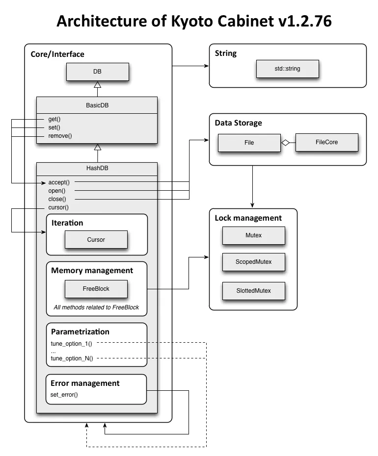
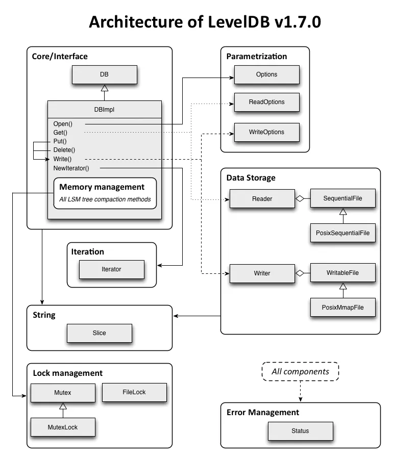
LevelDB 的核心（Core/Interface）更小，API 设计更紧凑。比方说，LevelDB 把参数也对象化，并通过 ReadOptions 和 WriteOptions 暴露读写操作，使得这些接口没必要与数据库的核心耦合起来。

Emmanuel 认为单独设计字符串的操作类 String 是有必要的，比如说 LevelDB 使用“Slice”来存储字符串可以把获取字符串长度降低到 O(1)（对比 strlen 在 C 中是 O(n) 的性能）。“Slice” 在拷贝时使用浅拷贝而不是深拷贝，使得它和 C++ 中 std::string 的表现不一致。总的来说，LevelDB 的 String 可以节约拷贝和分配内存的时间。而 KC 完全依赖 std::string。

KC 使用 C 风格的错误处理，在任何出错的地方返回数值异常值；LevelDB 没有使用异常捕获，而是使用了一个 Status 对象来标记程序运行正常或否（手动破折号）由于每个方法都有从返回值中判断错误情况，所以每个方法的调用都会多消耗一些内存。不过这种消耗是有意义的，它避免了魔法数值，并且将错误码和核心解耦。

在内存管理上两者有很大区别：KC 持续跟踪由 mmap() 映射的空闲内存块，并将数据储存到足够大小的块中。LevelDB 使用 LSM 树进行数据管理，一旦其大小超过一定阈值，便开始压缩。这两个数据库都是用文件系统储存数据。

IKVS Part 4 - API Design

Emmanuel 决定把自己的 KV Store 叫做 KingDB。在设计 API 时，他建议遵循 Joshua Bloch 的原则（以及 Effective C++）：

• 存疑则不留：不知道一个 API 是否应该暴露给用户时，不要暴露；
• 能做则做：如果客户端需要连续调用好几个函数来完成操作，那么将其包含进 API 中会使客户端更省事儿；
• 遵循传统：使 API 看起来像经典的应用，这能使客户端看一眼就知道怎么调用；

好的 API 应该对称：如果我调用了“open”，那应该还可以调用“close”，而不是像 LevelDB 一样使用 delete 来关闭数据库。同样，基于对称性的理由，Emmanuel 认为 API 中的 Get()/Put() 会比 Get()/Set() 更更易读一些；使用迭代器而不是游标来获取数据也是依此为据。

/* LevelDB */
leveldb::DB* db;
leveldb::DB::Open(leveldb::Options, "/tmp/testdb", &db);

leveldb::Iterator* it = db->NewIterator(leveldb::ReadOptions());
for (it->SeekToFirst(); it->Valid(); it->Next()) {
  cout << it->key().ToString() << ": "  << it->value().ToString() << endl;
}
delete it;

delete db;

KC 和 LevelDB 使用了两种完全不同的设定方法（见架构图）。给 KC 数据库实例设置参数时可以直接调用其方法；而 LevelDB 在设定参数时，需要创建新的参数对象，这样可以方便地在多个数据库之间共享对象。不过 LevelDB 每次 Get 或 Put 时都需要将参数对象作为第一个参数传入，Emmanuel 认为这样做也许有其理由，但是使用重载或是将参数对象作为最后一项可选参数要更“C++-style”一些。

IKVS Part 5 - Hash table implementations

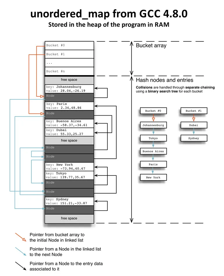
哈希表可以高效存取数据，但是在实际使用时，需要考虑许多值哈希后可能会得到一个结果，这时需要如何存储。为了解决哈希碰撞，常常使用链表或自平衡树来储存值，或使用线性或平分寻址技术。好的哈希算法应该使结果尽可能均匀地分布在索引数据范围内，比如 MurmurHash3、CityHash。

libstdc 中的 unordered_map 哈希算法使用链表实现了存储，它定义了“Node”结构用来保存当前节点的值以及下一个节点的地址。

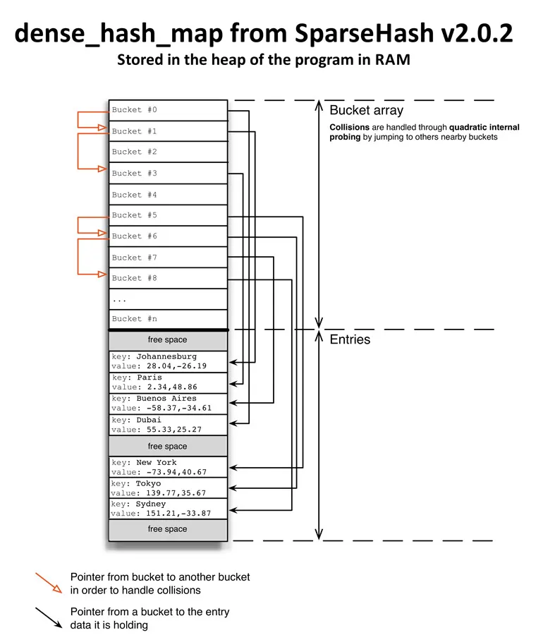
dence_hash_map 使用平分寻址技术来检测是否有空位。这种技术能较高效利用缓存以快速寻址，且能避免线性寻址容易造成的集群现象。

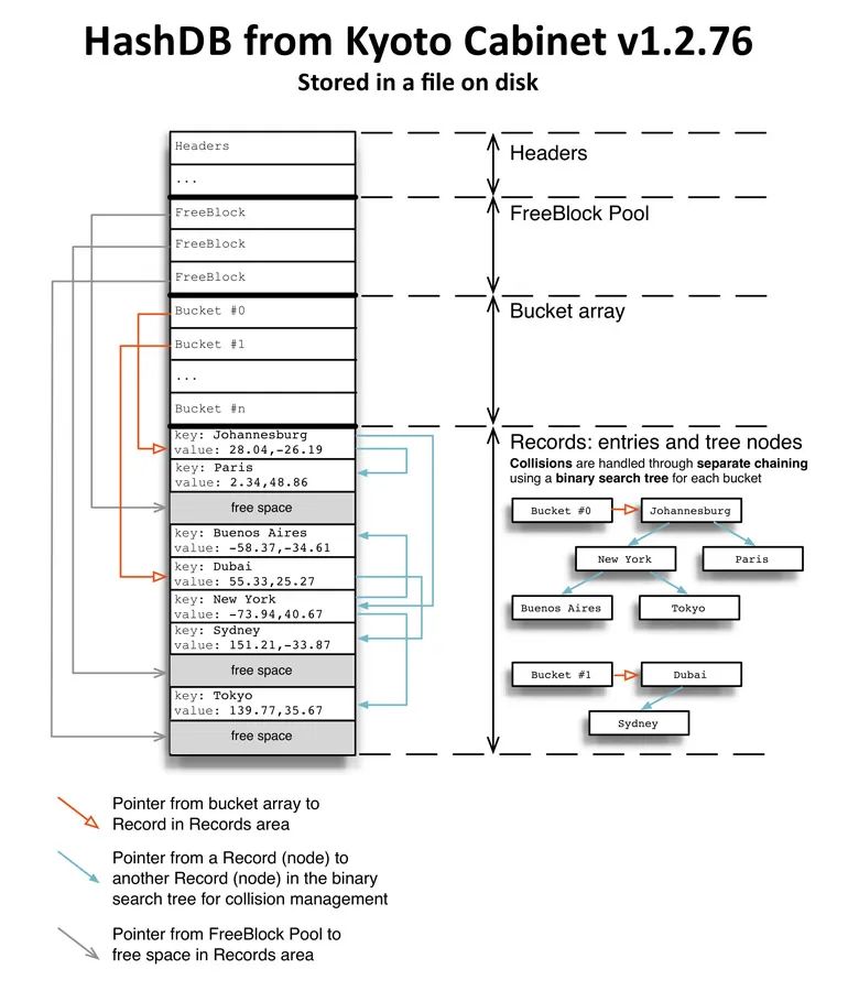
KC 使用了自己实现的哈希表 HashDB，它使用二分搜索树来储存数据。HashDB 分为四块，见下图，Header 用来存放数据库元信息，FreeBlock Pool 用来标记是否磁盘剩余的空间，Bucket Array 是索引数组，Records 则用来存放数据。由于 KC 的桶大小不能进行变更，所以一但其大小设置地比实际需要的更小，那么当桶快满时，KC 的性能就会开始急剧下降。

每个 Record 都需要记录以下信息。

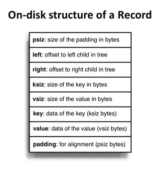
• psiz：填充的空白的大小
• left：搜索树的左节点偏离量
• right：搜索树的右节点偏离量
• ksiz：键的大小
• vsiz：值的大小
• key：键
• value：值
• padding：空白

可以发现，每个 Record 都是搜索树的一个节点。将树的节点和键值对用同一个结构储存下来是非常方便的做法，它使得储存不定长的数据成为可能，并且相比将两者分开存放能减少读盘次数。既然要用到搜索树，那么比较算法也是少不了的。KC 简单折叠了哈希值用于节点的排序：

/* from kyotocabinet-1.2.76/kchashdb.h */ 
uint32_t fold_hash(uint64_t hash) {
  return (((hash & 0xffff000000000000ULL) >> 48) | ((hash & 0x0000ffff00000000ULL) >> 16)) ^
    (((hash & 0x000000000000ffffULL) << 16) | ((hash & 0x00000000ffff0000ULL) >> 16));
}

IKVS Part 6 - Open-Addressing Hash Tables

Emmanuel 使用 DIP、DFB、DMB、DSB 等多个指标，重新对比了线性寻址、跳房子哈希和罗宾汉哈希的性能。由于 CPU Cache Line 的限制，DIB 等指标可能会在某些值附近出现性能突变的情况。也就是说，他们和性能并不是简单的线性关系。另外，作者还有一些感兴趣但没有列出的指标，比如：哈希冲突次数（这意味着额外的 IO 操作次数）和寄存器的缓存命中率。

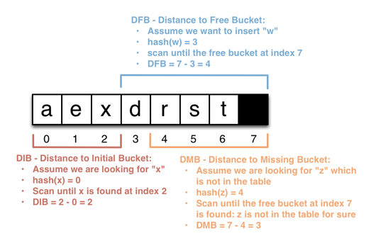
• DIB：Distance to Initial Bucket，指储存一个条目的位置到其键最初被散列到的位置的距离。
• DFB：Distance to Free Bucket，从给定入口到扫描到空位所跳过的数量。
• DMB：Distance to Missing Bucket，从给定入口扫描直到判断出该键不属于当前索引的扫描次数。
• DSB：Distance to Shift Bucket，在罗宾汉哈希中删除元素时如果使用某种算法会使综合性能提升，但会引入这个指标？？？
• Number of bucket swaps：罗宾汉哈希和跳房子哈希在插入后会重排序，会带来读写操作，所以需要考虑这个指标。

最终，得出罗宾汉哈希的性能要比跳房子哈希好许多。作者选用了罗宾汉哈希作为 KingDB 之后将实现的哈希表算法。

IKVS Part 7 - Optimizing Data Structures for SSDs

SSD 的基本原理和 HDD 有着巨大的不同。SSD 的基本更新单位是页，页的大小按照不同规格的储存器可能设计为 4KB、16KB 或是其它容量。这意味着，无论是多么小的数据，每次写入时都要按页写入。这浪费了许多写入性能，即写入放大效应。此外，SSD 通过内部的寄存器和 RAM 控制器来给出每一页设置过期标记，这割裂了储存的逻辑空间和物理空间。所以经典算法中的就地更新策略以及大于页容量级别的顺序读写算法，对于使用 SSD 作为储存介质的程序而言，只会徒增代码复杂度，不会带来任何性能提升。

普遍来说，SSD 的读取速度要远快于 HHD。所以针对 SSD 的程序的优化，通常是专注于写入。通常，SSD 的集群块（Clustered Block）的大小可以达到 32MB。由于内部的并行结构，对集群块的写入操作是十分快的（？）。依此原理，KingDB 需要尽量使用“追加”而不是“覆盖”的方式来一次性写入大量（集群块大小的）数据。

听起来好像到了 LSM-tree 擅长的领域？LSM-tree 通过建立了多级缓存，使写入以追加的形式写入快速缓存中；如果快速缓存慢了，比如达到了 32MB，再将缓存中的树合并为一颗更大的树，写入磁盘。假设 LSM-tree 有两级缓存，分别位于内存和 SSD 中，可以想象，它充分利用了内存的高速读写特性和 SSD 大批量写入时增速的特性。也即，LSM-tree 天然地把多次随机写操作推迟并合并成了在磁盘中的顺序写。当然，缺点也是有的。合并操作可能不可预测，且会造成突然的 CPU 高负载。

Emmanuel 还列举了几种围绕减少系统调用¹出现的优化 IO 的方法。

• 内存映射：使用内存映射相当于将文件区域映射为物理内存地址，这样一来，可以在程序中像操作缓存一样操作文件，而把 IO 操作留给系统内核优化及完成。
• 向量 IO：又称聚集发散 IO（scatter-gather I/O），不知是个啥。
• 零拷贝：见零拷贝。

IKVS Part 8: Architecture of KingDB

对相同值的索引，KingDB 直接使用新值去覆盖旧的值，而不是写入删除。这也就是为什么它的写入速度很快。所有的索引都使用 std::multimap 储存，分别记录 hashed key 和 location；索引有多个读取和一个写入，同时使用锁来保证在读取时索引不会改变。

Emmanuel 考虑过要实现自己的零锁版本的罗宾汉哈希，但是鉴于 std::multimap 能节约巨大的工作量，所以就直接用了。使用 std::multimap 带来的问题是：

• 需要经过两次哈希运算，手动计算哈希时一次，std::multimap 储存时本身需要对手动哈希得到的值在进行一次哈希。
• 索引需要完整的存入内存，这也就意味着数据库快照也需要占有许多内存。

KingDB 用 ByteArray 封装读取操作，它使用 RAII 以及内存映射技术提升性能。Another interesting point is that the data retrieved is likely to be larger than the maximum payload that can transit on a network, thus any type of caching while reading data from disk is going to increase the throughput. Memory maps are an easy way to get such caching, by reading only what is needed from the buffer and letting the kernel handle the caching. 因为储存在磁盘中的数据使用 LSM-tree 来保证在同一个区域不会同时有读写操作，所以 HSTable 中的内容可以访问时不加锁也没关系。

KingDB 被划分为了 Storage Engine 和 Server 两个部分，可以更方便测试。由于 Server 需要把接受到的所有数据都先放到新开辟的内存中再传到缓存，在传递大文件时很容易导致内存溢出，所以后来在 Write Buffer 和 Storage Engine 中引入了“Part” （应该是部分写入之类的概念）。同时，Server 需要完善 Multipart API（大文件分块接收与储存），而其中的权衡是：当客户端并发数很少时，revc() 允许客户端占用更大的缓存区，减少写入次数；如果并发多那么分块能使内存占用减少，但同时写入次数（以及相应的系统调用次数）就上去了。

写缓存（Write Buffer）把随机写入聚合起来，转换为一次更大的顺序写入,不过它的缺点在于可能会在大文件写入时造成写停顿（？？？）。见 Why buffered writes are sometimes stalled 。KingDB 有两个写缓存区，其中一个用于接受数据请求，另一个用做刷新操作的源（？？？）。当接受数据的缓存区准备好被刷新时，就会被锁定，然后两缓存区的角色互换。The two std::vector in the Write Buffer are storing instances of the Order class. Each order contains the key of the entry it belongs to, a part of data for the value of that entry, and the offset of that part in the value array. Keys and parts are instances of ByteArray, which allows to share allocated memory buffers when they are needed all along the persisting pipeline, and seamlessly release them once they have been persisted by the Storage Engine.

将所有可能等待 IO 操作的工作用多线程设计可以明显减少等待时间（downtimes）。Emmanuel 使用 C++11 的 std::mutex 来同步这些线程。尽管零锁版本可能是更优解，但是对于瓶颈在磁盘 IO 的 KingDB 来说，算过早优化了。如上图 KingDB 架构所示，其线程包含：

• Buffer Manager：用于控制缓存区与 Storage Engine 的交互。
• Entry Writer：等待 EventManager::flush_buffer 事件并处理从写缓存传入的 Orders Vector。
• Index Updater：等待 EventManager::update_index 并在合适的时机更新索引。
• Compactor：定期检查数据库的各项数据以确定是否需要调用压缩合并以回收磁盘空间。
• System Statics Poller：定期收集系统各项数据（如磁盘剩余容量）。

对于多线程间的消息通讯，KingDB 有自己的实现，仅 70 loc，使用 std::condition_variable 和 std::mutex 打造（源码见 KingDB/thread/event_manager.h）。如果线程间需要传输数据，那么就会使用到内部的事件系统。

异常管理还是沿用的 LevelDB 那套风格。KingDB 没有处理内存不足时的异常，作为内存数据库，对此异常无能为力。不过，KingDB 通过 Valgrind 详细检测了内存泄漏、堆破坏（Heap Corruption）、静态等项目。KingDB 使用 Status Class 而不是异常的原因是：

• Status 类更易读，可以容易分辨源码有没有明确地处理或是如何处理的错误；
• Exception 难以维护，想象一下为之前没有考虑过的错误情况添加或更改额外的异常类型；
• Code locality matters, and exceptions make everything they can to make that not the case — technically, exceptions are free as long as they are not thrown; when they’re thrown, they incur a 10-20x slowdown with the Zero-Cost model.

在调试时，可以把日志级别设置为“trace”，而在生产环境这设置为“error”。日志相关方法都是在 printf 基础上的封装。另一方面，参数类也是单独的封装。正如前文所描述的，将参数化对象封装起来有助于解耦核心引擎，这也是从 LevelDB 中习得的。

压缩算法选用了 LZ4，校验和算法是 CRC32，哈希算法可以从 Murmurhash3 以及 xxHash 中任选。

IKVS Part 9: Data Format and Memory Management in KingDB

IKVS Part 10: High-Performance Networking: KingServer vs. Nginx

Hash Collisions

Read More

USENIX ATC '20 - MatrixKV Reducing Write Stalls and Write Amplification in LSM-tree Based KV Stores

‍ Hello, everyone. My name is tian yao from hua zhong university of science and technology. ‍‍My talk today is metrics kv reducing right store and right amplification in lsmg based kv stores‍‍ with a metrics container in on the end. ‍‍This is a joint work of pink cup company, the university of texas at arlington and temple university. ‍‍I will give this talk in four parts. First, let me introduce the backgrounds and motivation. ‍‍L symmetry based akv store are widely deployed in riding tensive scenarios. ‍‍Popular kv stores such as level db cassandra and rocks db are built with l sm tree. ‍‍They usually run assistance with d ram and ssd storage is‍‍ elsam trees offer high ride throughput by batching right in memory and offer faster read and range quarries with lifetime compaction. ‍‍This figure present the structure of an l symmetry in the popular implementation, rocks db‍‍ rusty b is composed of ad ram component and an ssd component. ‍‍Alsome tree levels on ssd are exponentially increased from level zero to level six. ‍‍At the amplification factor of ten rights request, first inserting to memory tables in d ram, ‍‍then flush to ssd finally do level by level complexions. Overall, ‍‍the operations of rux db manly includes insert, flush and compassion of multiple levels‍‍ to better understand elm tree based the, kb store. ‍‍We evaluate rocks db by randomly writing an 80 gigabyte data set‍‍ and measure the random rights throughput in every 10 seconds. ‍‍From this figure, we first observe the challenge of right store. That is‍‍ application throughput periodically dropped to nearly zero. The troughs of system throughput indicate right stores, ‍‍the dramatic fluctuation of performance and long tail latencies‍‍ go against non sequel assistance, design goal of predictable and stable performance. ‍‍To figure out the reason of rice stores, we record the period of each flush and compaction‍‍ of different levels. Surprisingly, we find that the period of level zero to level one compaction‍‍ mattress right stall approximately. ‍‍Here we can see that each red line represent a level zero to level one compaction. ‍‍Its lands along x axis represent the latency of the compaction. ‍‍The right y axis shows the amount of data processed in each complexion. So‍‍ it reaches 3.1 gigabyte, on average. ‍‍Now we elaborate the level zero to level one compaction to explain why it involves so much compaction data‍‍ to come back a level zero to level one compaction. First, we pick a victim assets table in level zero. ‍‍Second, over left ss tables in level one are picked. Third, ‍‍since ss tables in level zero, are ov er la pp ed to each other. ‍‍We go back to level zero and pick more ss tables within the compaction key range. Fourth, we've‍‍ go to level one and find if there are any other ov er la pp ed as as tables and picks day and pick it. ‍‍Now we get all the compaction data or the compaction data, ‍‍or read into the memory, merge and salt, then right back to level one. ‍‍As we go back and forth between level zero and level one. ‍‍Almost ss all assets tables in both level, joins the level zero to level one compaction in the end. ‍‍The larger amount of compaction data leads to heavy read, ‍‍merge, right? Which takes up cp u cycles and ssd bandwidth, ‍‍thus blocking foreground request and making level zero to level one compaction, the primary cost of right stores‍‍ from the same test. We observe the second challenge. ‍‍As the green line shows, system throughput degrade with the increase of data sets, size. ‍‍The growing data set increases the depths of an l symmetry, so that brings more compaction and thus higher right amplification. ‍‍As we know, l symmetry based kv stores have long been criticized for their high right amplification, ‍‍due to level by level complexions with the amplification factor of adjacent levels of ten, by default. ‍‍Right? Amplification increases with a number of levels. ‍‍That is right, amplification accords to af times n where n is the number of levels. ‍‍Emerging non voluntal memory technologies has the property of fast success by adjustable and persistency. ‍‍It provides us a potential solution to adjust the both challenges. ‍‍Na va sm from abc 18 adopts only m to store large mutable memory tables. ‍‍From the right figure, we can see that now vs m improves random right throughput‍‍ compared to rocks. Db is about 1.7 times. ‍‍To some extent, it due reduce right amplification. ‍‍However, it significantly increases the size of on sorted level zero. ‍‍That makes level zero to level one. Compassion data reaches 15 gigabyte. ‍‍The larger amount of compassion data making the period of right store extended severely. Hence, we say‍‍ the state of art solution. ‍‍Now, sm is not sufficient to adjust the both two challenging issues. ‍‍From the above analysis, we conclude that‍‍ all to all level zero to level one, compaction is the main cause of red stock. ‍‍Rice stop brings unpredictable and unstable performance. ‍‍The increased depth of alexum tree is the main course of increased, right amplification. ‍‍Higher, right? Amplification brings decreased system performance, especially decreased random, right? Throughput, ‍‍motivated by these challenging issues. ‍‍We propose matrix kv‍‍ that aims to reducing right store and right amplification in l symmetry based kv stores by exploiting nvn‍‍ next, we will see the design of metrics, kv‍‍ this figure shows the overall architecture of matrix kv we add an nvm between d ram and ssd‍‍ as we can see from the right figure from the top to the button, they ran batches, right? ‍‍Nvm stores the top level of sm tree with our proposed metrics container. ‍‍Ssd stores the remaining levels of a flattened alison tree. ‍‍Matrix kv has four design strategies. First, the metrics container in nvn that stores‍‍ and manage the un. So rt, ed level zero. Second, the column compaction to reduce right stores. Third, ‍‍the flattened sm tree on ssd to reduce right amplification‍‍ and force the crossroad hint search to improve the red efficiency in nvn‍‍ in the following, I will introduce all the four design strategies, one by one. ‍‍First, let's see the metrics container manages the level zero of lsm three. ‍‍He consists of a receiver and a compactor. ‍‍For receiver, it receives flushed memory table from the ram and stores them row by row, ‍‍where each row is organized as a role table. As showing this figure, ‍‍an immutable memory table flashed from the rain is stored in the receiver as a row table. ‍‍Once the receiver is fully filled, in process, a it logically turns into a compactor. ‍‍Then‍‍ for competitor, it compacts data from level zero to level one column by column. ‍‍We call it column compaction like these. The nvm pages of a, column or freed after the column compaction. ‍‍Those 3 pages are returned to the free list and waiting for storing newly flashed data. ‍‍Here we show the row table structure. Row table consists of data and math data. ‍‍The data region stores serialized kv items from the immutable memory table. ‍‍The math data region is a sorted array. ‍‍Isury, my element maintains the key, the page number, the offsetting the page, ‍‍and a forward pointer for crossroad hint search. To locate akv item in this row table. ‍‍We just need binary search, the sorted array to forget the target key, ‍‍and then its value can be indexed with the page number and offset‍‍ with the metrics, container and road table. ‍‍Now we can do, ‍‍we can do the fine grand column compaction for level zero and level one. ‍‍The non ov, er la pp ed level one on ssd provide us assorted key space with multiple contiguous key ranges. ‍‍As showing this figure, the contiguous key range are 023, ‍‍325528, and so on. ‍‍Now I introduce the column compaction with an example. ‍‍Column compassion starts from the first key range in level one that is 0 to 3, then‍‍ multiple thread in the compactor or‍‍ multiple threats in the compactor searches, the keys within the key range, 0 to 3 like this. ‍‍If the amount of data is under the threshold of a compaction, the next key range 3 to 5 joins, ‍‍if the amount of data is still not enough, the next range 5 to 8 joins. ‍‍Finally, the compaction range is 0 to 8. ‍‍A logical column is formed with the data within the key range, 0 to 8. ‍‍And the column compaction merges the column and the first two ss tables in level one. ‍‍Then we do the next column compaction, arrange 8 to 30 and the next one‍‍ by processing level zero to level one, column, compassion, column by column. ‍‍Each compaction only merges a small key range that has very limited amount of data. Hence, ‍‍the column compaction can reduce right amplification, right? Stores due to all compaction. ‍‍Since right amplification, ecles to af times the number of lmc levels‍‍ matches kb tries to flatten the lcm tree to reduce right amplification. ‍‍So‍‍ what we do is keep the af on change while increasing the size of level zero and level one to reduce the n‍‍ due to column compassion, the size of level zero and level one does not affect the overhead‍‍ of level zero to level one. Compaction is always at a limited amount of data. ‍‍Since larger on salted level zero might decrease. ‍‍The red efficiency of metrics, kv we propose crossroad hint, search next. The process of crossroad hint, search. ‍‍To process the crossroad hint search, we need construct, crossroad hint with forward pointers. First. ‍‍For the key x in row table I is forward point indexes the key y in row table I minus one. ‍‍Why always the first key that no less than x‍‍ for example, here, 3 points, 235.267points to 8, and so on. ‍‍In this way, we can logically sort all keys in level zero. ‍‍Now, ‍‍if you want to search the key 12, ‍‍we first binary search, the row table three to get two adjacent keys. We wear. ‍‍The 12 might recite that is p 10 and 23 with the forward pointer of 10 and 23. ‍‍We can go to round table, too. ‍‍The key aid is added into our search region, because 12 is between 8 and 13. Then‍‍ we will go to row table one with the forward pointer of key 8 and 13. ‍‍Then we go to let row table zero finally, and find 12 in row table zero. ‍‍From this yellow region, we can see that crossroad hinge search‍‍ compares fewer keys that's reducing the search overhead compared to travels all of the keys and‍‍ come compares, all of the keys. ‍‍For the evaluation, we compare matrix kb with conventional rocks cb‍‍ which is the ssd based rock cb and the rock cb level zero in the end, ‍‍where it put level zero in nvm and run assistance with d ram mvmssd hierarchy, ‍‍then is the state of art. ‍‍Now, sm all the systems use‍‍ eight gigabyte opton, dcpmm‍‍ this figure shows the random right throughput with value sizes, ranging from 64 byte to 64 kilobyte. ‍‍Generally, matrix kv obtains the best random performance in all the different value sizes. ‍‍We just take the four kb value size as an example metrics. Kv out performs roxy b level zero and vn‍‍ by 3.6 times. And out performs not sm by 2.6 times respectfully. Next, ‍‍we will in explain this advantage of metrics. Kv comes from two reason. ‍‍The first is reduced the right store. The second is decreased, right amplification‍‍ by recording the throughput in every 10 seconds during the 80 gigabyt random note. ‍‍We see the fluctuation of system performance. Here, metrics kv is represented by red line. ‍‍This figure show that mattress kv is the fastest to load the same at gigabyte data set. ‍‍It has the most stable random right throughput, which means‍‍ we do reduce right stars with column compaction. ‍‍Okay? ‍‍In terms of tale latency, we can see that matrix kv obtains the shortest tale latency in all cases. ‍‍Taking the 99 person tale latency as an example. ‍‍Mattress kv is 27 times lower than rocks dbssd 5 times lower than not sm‍‍1.9 times lower than rocks db level zero nvn‍‍ here, we record each level zero to level one compaction to explain why matrix kv reduce right stores. ‍‍From this figure, we can see that for each level zero to level one compaction. Now, sm merges‍‍15 gigabyte data. Now sms rock cbssd merges 3.1 gigabyte data, ‍‍rock cb level zero nvn merges 4.9 gigabyte data. However, ‍‍metrics kv only merges 33 megabyte data, and it‍‍ due the column compaction for 467 times. So‍‍ the small but multiple time compaction reduce right store. ‍‍Here we show the right amplification of randomly loading 80 gigabyte data set. Test result show that‍‍ by flattering, the l symmetry matches kv reduces right amplification than others resistance. That's‍‍ that is 3.43 times here, right? Amplification is calculated by the ratio of‍‍ amount of data riden to ssd‍‍ to amount of data written by users. ‍‍In summary, conventional ssd based kv store are‍‍ has unpredicted has unpredictable performance due to write stores‍‍ And decrease the performance due to higher, right? Amplification. ‍‍Matches kv build an l symmetry based kv store for assistance with d RM, ndm and SSD storage. ‍‍With four design strategies, metrics, KB reduces right store and improves right throughput. Finally. ‍‍Thanks, everyone.